Technology
技術分享
Intelligent Lump-Sum Engineering Optimized Performance of a Plant
Dynamic Simulation Analysis of Steam Distribution Networks
Through technological developments and innovations, CTCI has taken the lead in offering enhanced iEPC intelligent lump-sum engineering services. By introducing a dynamic simulation analysis of steam distribution networks to refinery and petrochemical engineering and cooperating with the Department of Chemical Engineering at National Taiwan University, CTCI has enabled global customers access to innovative overall plant operations and energy consumption.
The steam system is a key energy carrier in a chemical plant. It provides shaft work to rotating machines and thermal energy to heating equipment, and also integrates thermal energy between different operational units. Therefore, analysis via a dynamic simulation can be used to verify the design of steam distribution networks to identify potential issues prior to construction. Subsequently, it contributes to avoiding extensive shutdowns, thus insuring consistent steam quality while improving the energy efficiency of steam distribution networks and the overall plant.

However, there were many factors influencing the operation of steam distribution networks. For instance, the size and length of the piping, the thickness and efficacy of thermal insulation material, the operating flow rate, and the temperature and pressure can all affect energy dissipation, proper operations, and safety. Hence, it is difficult to simulate and analyze large scale steam distribution networks, considering a steady state and dynamic temperature and pressure trends as the flow rate may vary. This article applied a looped-network system, combining with the cycling implicit and the Hardy Cross methods to simulate and analyze a large-scale steam network in a petrochemical plant for CTCI.
Looped-network steam distribution system
In general, steam distribution networks fall into two categories: branch systems (Figure 1) and looped-network systems (Figure 2). In Figure 1, the blue arrows represent sources of supply, while the red arrows represent consumption sinks and the green points are nodes.
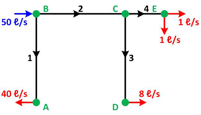
Figure 1. Branch system
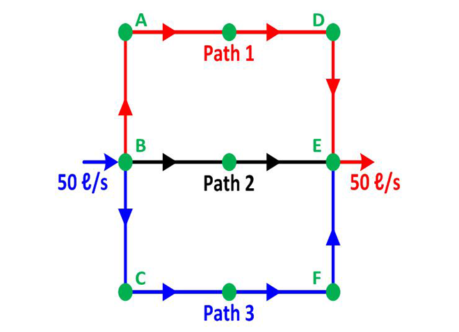
Figure 2. Looped-network system
When a user wishes to move steam from Node B to Node A in Figure 1, only one path is available in a branch system, which is B→C→E. In Figure 2 , three paths, namely B→A→D→E, B→E, and B→C→F→E can be selected based on certain considerations. In the looped-network system, if some upset or maintenance occurs in one path or supply, steam will continue to be compensated via other paths. This is the major difference between a branch and a looped-network system. On the other hand, a branch system can be considered as a special case of a looped-network system. Thus, this article only considers the analytic method for looped-network systems.
Two mathematical calculation methods
1.Looped-implicit method

Steam transportation is a compressible flow system with heat transfer. The governing equations include: the continuity equation, conservation of momentum, and the conservation of energy. Some correlations, such as the friction factor between the Reynolds number and roughness as well as energy dissipation between insulation materials, need to be considered, too. An important issue is how to use appropriate analytical mathematical methods to solve these complex hyperbolic partial differential equations. This article briefly outlines these issues.

Two common techniques used are the characteristic and the implicit methods. Each one has its own advantages and disadvantages. The characteristic method transforms simultaneous hyperbolic partial differential equations into matrix form to derive a solution. The implicit method substitutes functional variables and solves them using the Newton method. Due to the characteristic method’s restrictions, it cannot perform calculations for larger time intervals. Thus, it would takes more time when applied on a large-scale network. However, it can present detailed variations of temperature and pressure in short time intervals when applied on a process that is changing rapidly. The speed of calculation and the convenience can be enhanced by a looped-iteration procedure, making it more suitable to simulate large-scale steam distribution networks.

2.Hardy Cross method

Hardy Cross has been reported as an analytical method based on material and head balance used for the evaluation of the flow distribution of water networks. Wang et al proposed a modified version of the Hardy Cross method which takes into account compressible flow with heat transfer. This method is still based on material balance (Equation 1) and the summation of pressure in loops is zero (Equation 2, where M [kg/s] is the mass flow rate of steam).

Equation 2 represents the steady-state condition. For solving the steady steam flow rates, a correction factor of flow rateΔMk (Equation 3) is introduced to each loop k. Rearrangement of Equation 3 will derive Equation 4 forΔMk . This factor is used to correct the flow rate of loop k. Steady flow rates are evaluated by iteration untilΔMk is less than the tolerance in every loop.
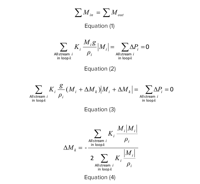
In short, the concept of the Hardy Cross method for compressible flow is as follows:

1.Number every pipe segment, node, loop and supply. Assume clockwise direction as positive.
2.Estimate the flow rate of each pipe segment based on material balance.
3.Calculate Ki for each pipe segment.
4.Calculate the flow correction factorΔMk for each loop k via Equation 4.
5.Add correction factorΔMk to the flow rate of each loop k and calculate the corrected flow rate of every pipe segment.
6.Iterate from step 4 until the correction factor ofΔMk of all loops is less than the tolerance. This calculated flow distribution is the steady condition.
Dynamic simulation of steam distribution networks in a petrochemical plant
Figure 3a is the scheme of a single-loop high-pressure steam network in a petrochemical plant. 8 red squares indicate high-pressure steam supply sources, including 3 high pressure steam boilers, which supply roughly 60% of high pressure steam for the plant. 11 blue squares represent various users. Pipe segments have more parameters, so they were temporarily omitted. Figures in squares represent the initial condition of high-pressure steam for every supply or user. The gray figures next to the pipe represent the number of pipe segments. Green arrows represent the flow direction of the steam. Black figures next to the arrows indicate the steam flow rate.

Figure 3a reveals a quite complex steam distribution of the original steady state. For example, in the case of the 101 ton/h high-pressure superheated steam (42.2 atm, 683.6 oC), 52.6 ton/h flows to the left while 48.4 ton/h flows to the right. For 52.6 ton/h high-pressure steam on the left-hand side, 40 ton/h is combined with 36 ton/h steam from unit 4 and supplied to unit 1. The remaining steam is supplied to units 2 and 3. Meanwhile, 48.4 ton/h of steam on the right-hand side is combined with 71 ton/h of steam from unit 5, and supplied to unit 6 (94 ton/h). The remaining 25.4 ton/h of steam is supplied units 7, 14, 15, and 16 together with steam from the second boiler. While the required high-pressure steam of unit 3 is entirely supplied by the first boiler, the adjacent unit 2 was supplied mostly by the third boiler.
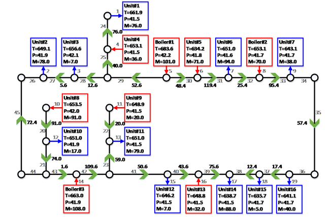
Figure 3(a). Scheme of a high-pressure steam network in the case of a petrochemical plant: Initial steady condition
If such a petrochemical plant were to repair the third boiler due to accident, maintaining the other units under normal operations would mean steam originally supplied by the third boiler is required to be compensated by the other supply nodes (mainly the first and second boilers) in order to satisfy all original steam requirements. The key points are differences in dynamic trends and the impact on each unit between 108 ton/h of steam which is compensated by the first or second boiler.

1.First operating scenario

In the first operating scenario, the 108 ton/h originally supplied by the third boiler is compensated by the first boiler. Figure 3b shows the new steady state under such a condition.
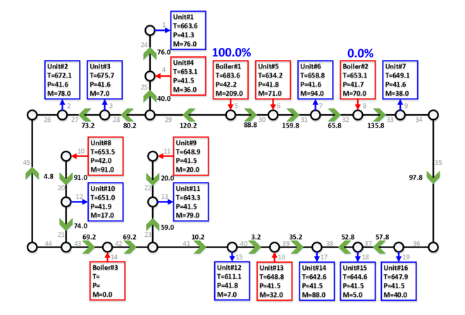
Figure 3(b). Scheme of a high-pressure steam network in the case of a petrochemical plant: New steady state of the first boiler compensating for 100% of insufficient steam
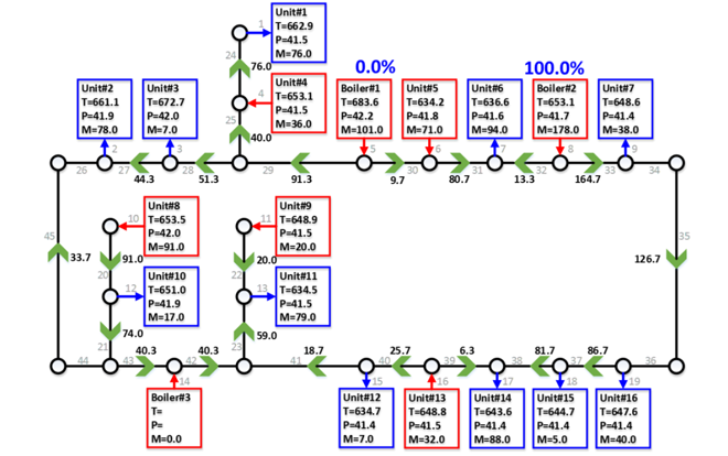
Figure 3(c). Scheme of high-pressure steam network in the case of a petrochemical plant: New steady state of the second boiler compensating for 100% of insufficient steam
2.Second operating scenario

In the second operating scenario, the 108 ton/h originally supplied by the third boiler is compensated by the second boiler. Figure 3c shows the new steady state under this scenario.

Figure 4a-c shows the temperature trend of units 1, 6, and 11 under different ratios of insufficient steam compensated by the first or second boiler. The percentages represent the ratio of 108 ton/h of insufficient steam from the first boiler. In Figure 4a, although the temperature of unit 1 finally rises as the loading of the first boiler decreases, the range of temperature raised and oscillation decreased.
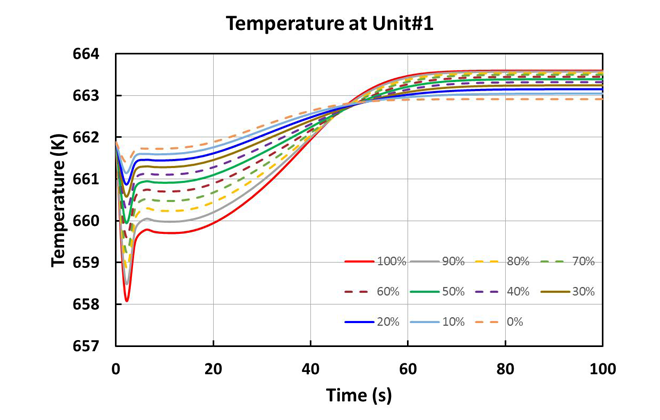
Figure 4(a). Temperature trend of unit 1 under different ratios of steam compensated by the first and second boilers
In Figure 4b, for unit 6, the final temperature raised while the ratio of steam is compensated by the first boiler decreases from 100% to 40%. In the range from 40% to 0, the final temperature declines.
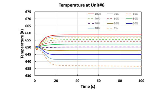
Figure 4(b). Temperature trend of unit 6 under different ratios of steam compensated by the first and second boilers
In Figure 4c, for unit 11, the final temperature consistently declines. However, the amount of the decline and the required time to reach the final steady state increases.
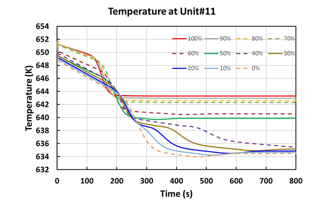
Figure 4(c). Temperature trend of unit 11 under different ratios of steam compensated by the first and second boilers
Optimized iEPC services through innovative technologies to enhance the performance of petrochemical plants
In this article, the looped-network example simulated and analyzed the case of a petrochemical plant. According to the simulation results, the temperature and pressure trends versus time were helpful in selecting the proper operating method.

In the case of a petrochemical plant, a viable operating strategy was associated with 70% compensating steam from the first boiler and 30% from second boiler, assuming the operating requirements were less oscillating of unit 1 as the flow rate varied and the temperatures of units 11 and 6 were prevented from falling too much.

In order to bring such new benefits of operating a plant overall and saving on energy consumption, CTCI has introduced a dynamic simulation analysis of steam distribution networks to refinery and petrochemical engineering. The use of innovative technologies to enhance iEPC intelligent lump-sum engineering services goes a long way to make CTCI the most reliable global engineering services provider.